santaR Theoretical Background

santaR is a Functional Data Analysis (FDA) approach where each individual’s observations are condensed to a continuous smooth function of time, which is then employed as a new analytical unit in subsequent data analysis.

santaR is designed to be automatically applicable to a high number of variables, while simultaneously accounting for:

biological variability
measurement error
missing observations
asynchronous sampling
nonlinearity
low number of time points (e.g. 4-10)

This vignette focusses on the theoretical background underlying santaR and will detail:

Concept of Functional Data Analysis
Main hypothesis
Signal extraction using splines
Group mean curve fitting
Intra-class variability (confidence bands on the Group mean curves)
Detection of significantly altered time-trajectories

Concept of Functional Data Analysis

Traditional times-series methodologies consider each measurement (or observation) - for example a metabolic response value at a defined time-point - as the basic representative unit. In this context, a time trajectory is composed of a set of discrete observations taken at subsequent times. Functional data analysis¹ ² ³ is a framework proposed by Ramsay and Silverman which models continuously each measured values as variable evolves (e.g. time). Contrary to traditional time-series approaches, FDA consider a subject’s entire time-trajectory as a single data point. This continuous representation of the variable through time is then employed for further data analysis.

More precisely, FDA assumes that a variable’s time trajectory is the result of a smooth underlying function of time which must be estimated. Therefore, the analysis’ first step is to convert a subject’s successive observations to the underlying function \(F(t)\) that can be evaluated at any desired time values

Two main challenges prescribe the exact characterisation of the true underlying function of time \(F(t)\). First, the limited number of discrete observations constrains to a finite time interval and does not cover all possible values, while the true underlying smooth process is infinitely defined. Secondly, intrinsic limitations and variabilities of the analytical platforms mean that the discrete observations are not capturing the true underlying function values, but a succession of noisy realisations.

A metabolite’s concentration over the duration of the experiment is the real quantity of interest. As the true smooth process \(F(t)\) cannot be evaluated, due to the collection and analytical process only providing noisy snapshots of its value, an approximation of the underlying metabolite concentration \(f(t)\) must be employed. This approximation can be computed by smoothing the multiple single measurements available.

The approximation of the underlying function of time, of a single variable observed on a single subject, is generated by smoothing \(y_i\) observations taken at the time \(t_i\), such as:

\[y_{i}=f(t_{i})+\epsilon_{i}\]

Where \(f(t)\) is the smoothed function that can be evaluated at any desired time \(t\) within the defined time domain, and \(\epsilon_i\) is an error term allowing for measurement errors. By extension, if \(f(t)\) is defined as representing the true variable level across a population, \(\epsilon\) can allow for both individual specific deviation and measurement error.

In order to parametrise and computationally manipulate the smooth approximation, the representation is projected onto a finite basis, which expresses the infinitesimally dimensional \(f(t)\) as a linear combination of a set of basis functions. A wide range of basis functions (e.g. polynomials, splines, wavelets, Fourier basis) are available, even if the most commonly used are Fourier basis for periodic data and splines for aperiodic trajectories⁴.

Following smoothing, a time-trajectory is expressed as a linear combination of a set of basis functions, for which values can be computer at any desired time without reconsidering the discrete observations. It is assumed that, if a satisfactory fit of the original data is obtained, both the new smooth approximation and the preceding noisy realisations should provide a similar representation of the underlying process⁵ ⁶

In practice, by assuming and parametrising (explicitely or implicitely) the smoothness of the function and leveraging multiple measurements in time as well as multiple individual trajectories, the smoothed representation can implicitly handle noisy metabolic responses. Additionally, as functional representations do not rely on the input data after their generation, smoothing approaches can handle irregular sampling and missing observations, translating to trajectories that can be compared without requiring missing values imputation. As such, the FDA framework and the smoothness assumption provide the necessary tools for the time-dependent analysis of short and noisy metabolic time-trajectories.

Main hypothesis

The working hypothesis is that analyte values are representative of the underlying biological mechanism responsible for the observed phenotype and evolve smoothly through time. The resulting measurements are noisy realisations of these underlying smooth functions of time.

Based on previous work performed in Functional Data Analysis, short time evolutions can be analysed by estimating each individual trajectory as a smooth spline or curve. These smooth curves collapse the point by point information into a new observational unit that enables the calculation of a group mean curve or individual curves, each representative of the true underlying function of time.

Further data analysis then results in the estimation of the intra-class variability and the identification of time trajectories significantly altered between classes.

Signal extraction using splines

Fitting splines to time trajectories is equivalent to a denoising or signal extraction problem: balancing the fitting of raw data versus the smoothing of the biological variability and measurement errors. Splines are piecewise polynomials with boundary continuity and smoothness constraints, which require a minimum of assumptions about the underlying form of the data⁷ ⁸ ⁹. The complexity of the fit is controlled by a single smoothing parameter \(\lambda\).

The data \(y_{ij}\) of individual \(i\), \(i=1,.,n_k\), observed at time points \(t_{ij}\), \(j=1,.,m_i\), in a group of \(n_k\) individuals, is modelled by a smoothing spline \(f_i(t_{ij})\) of continuous first and second derivatives that minimizes the penalized residual sum of squares (PRSS) (Eq. 1):

\[PRSS(f_{i},\lambda)=\sum_{j=1}^{m_{i}} \{y_{ij} - f_i(t_{ij})\}^2 + \lambda \int_{t_{min}}^{t_{max}}\{\ddot{f_i(t)}\}^2~dt\] (Eq. 1)

The first term of Eq. 1 is the squared error of employing the curve \(f_i(t)\) to predict \(y_{ij}\), measuring the closeness of the function to the data. The second term penalises the curvature of the function while \(\lambda\) controls the trade-off between both terms. The smoothing parameter \(\lambda\) is shared among all individuals. The monotonic relationship between the smoothing parameter \(\lambda\) and the desired equivalent number of degrees of freedom (df) of the corresponding fit (Eq. 2), allows us to control the closeness of curve fitting by varying df¹⁰.

\[df_{\lambda}=trace(S_{\lambda})\] (Eq. 2)

where \(S_{\lambda}\) is the smoother matrix (roughness matrix, or hat matrix) which transforms the observed data vector to the vector of fitted values (for more information see Eubank¹¹, and Buja et al.¹²).

The df parameter controls how closely the spline fits the input data. For example, when df is minimal (df=2), the smoothing is maximised and the original data points fitted with a straight line. On the other hand, when df approaches the number of time-points, every data point is fitted without smoothing, which can result in an over-fit of the raw measurements.

library(ggplot2)
library(gridExtra)
library(grid)

# Sample a gaussian distribution, add noise to it
x       <- c(-4, -3, -2, -1.5, -1, -0.5, 0, 0.5,  1, 1.5, 2, 3, 4)
y       <- dnorm(x, mean = 0, sd = 1, log=FALSE)
y_noise <- jitter(y, 90)

# Fit different smoothing splines, project on a grid for plotting
time     = seq(-4, 4, 0.01 )
tmp_fit0 = smooth.spline(x, y, df=13)
tmp_fit1 = smooth.spline(x, y_noise, df=2)
tmp_fit2 = smooth.spline(x, y_noise, df=5)
tmp_fit3 = smooth.spline(x, y_noise, df=13)

pred0    = predict( object=tmp_fit0, x=time )
pred1    = predict( object=tmp_fit1, x=time )
pred2    = predict( object=tmp_fit2, x=time )
pred3    = predict( object=tmp_fit3, x=time )

tmpPred0 = data.frame( x=pred0$x, y=pred0$y)
tmpPred1 = data.frame( x=pred1$x, y=pred1$y)
tmpPred2 = data.frame( x=pred2$x, y=pred2$y)
tmpPred3 = data.frame( x=pred3$x, y=pred3$y)

tmpRaw   = data.frame( x=x,  y=y)
tmpNoisy = data.frame( x=x,  y=y_noise)

# Plot original data and spline representations
p0 <- ggplot(NULL, aes(x), environment = environment()) + theme_bw() + xlim(-4,4) + ylim(-0.1,0.5) + theme(axis.title.y = element_blank(), axis.ticks = element_blank(), axis.text.x = element_blank(), axis.text.y = element_blank(), plot.margin=unit(c(0.5,0.25,0.5,0), "cm"))
p0 <- p0 + geom_point(data=tmpRaw, aes(x=x, y=y), size=1.5 )
p0 <- p0 + geom_line( data=tmpPred0, aes(x=x, y=y), linetype=1, color='springgreen3' )
p0 <- p0 + xlab(expression(atop('True underlying', paste('function of time'))))

p1 <- ggplot(NULL, aes(x), environment = environment()) + theme_bw() + xlim(-4,4) + ylim(-0.1,0.5) + theme(axis.title.y = element_blank(), axis.ticks = element_blank(), axis.text.x = element_blank(), axis.text.y = element_blank(), plot.margin=unit(c(0.5,0.25,0.5,-0.25), "cm"))
p1 <- p1 + geom_point(data=tmpNoisy, aes(x=x, y=y), size=1.5 )
p1 <- p1 + geom_line( data=tmpPred1, aes(x=x, y=y), linetype=1, color='blue' )
p1 <- p1 + xlab(expression(atop(lambda*' -> '*infinity, paste('DF = 2'))))

p2 <- ggplot(NULL, aes(x), environment = environment()) + theme_bw() + xlim(-4,4) + ylim(-0.1,0.5) + theme(axis.title.y = element_blank(), axis.ticks = element_blank(), axis.text.x = element_blank(), axis.text.y = element_blank(), plot.margin=unit(c(0.5,0.25,0.5,-0.25), "cm"))
p2 <- p2 + geom_point(data=tmpNoisy, aes(x=x, y=y), size=1.5 )
p2 <- p2 + geom_line( data=tmpPred2, aes(x=x, y=y), linetype=1, color='blue' )
p2 <- p2 + xlab(expression(atop('Optimal '*lambda, paste('Optimal DF', sep=''))))

p3 <- ggplot(NULL, aes(x), environment = environment()) + theme_bw() + xlim(-4,4) + ylim(-0.1,0.5) + theme(axis.title.y = element_blank(), axis.ticks = element_blank(), axis.text.x = element_blank(), axis.text.y = element_blank(), plot.margin=unit(c(0.5,0.25,0.5,-0.25), "cm"))
p3 <- p3 + geom_point(data=tmpNoisy, aes(x=x, y=y), size=1.5 )
p3 <- p3 + geom_line( data=tmpPred3, aes(x=x, y=y), linetype=1, color='blue' )
p3 <- p3 + xlab(expression(atop(lambda*' = 0', paste('DF = N'))))

grid.arrange(p0,p1,p2,p3, ncol=4)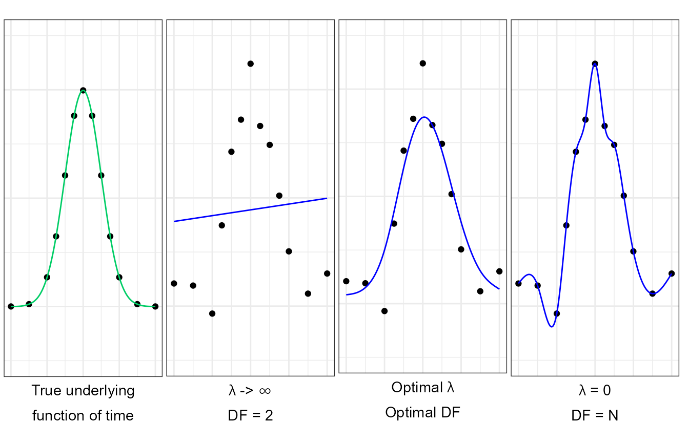

Multiple smoothing-spline fits of noisy realisations generated from a true smooth underlying function of time . A true smooth underlying function (continuous green line) is observed at multiple time points (dots). Noise is added to these measurements and the underlying function is approximated using smooth-splines at multiple levels of smoothness (blue continuous line).

Excessive smoothness makes the fit less sensitive to the data, resulting in an under-fitted model.

When the curvature is not penalised an interpolating spline passing exactly through each point is selected, resulting in an over-fitted model.

At intermediate levels of smoothness, a compromise between the goodness-of-fit and model complexity can be achieved, generating a satisfactory approximation of the true underlying function of time.

In practice, the results are resilient to the df value selected across all variables, which is a function of the study design, such as the number of time-points, sampling rate and, most importantly, the complexity of the underlying function of time. While an automated approach cannot infer the study design from a limited set of observations, an informed user will intuitively achieve a more consistent fit of the data.

santaR considers df as the single meta-parameter a user must choose prior to analysis, balancing the fitting of raw observations versus the smoothing of the biological variability and measurements errors. In turn, this explicit selection of the model complexity reduces the execution time and increases the reproducibility of results for a given experiment and across datasets.

For more information regarding the selection of an optimal value of df see the vignette ‘Selecting an optimal number of degrees of freedom’

Group mean curve fitting

Individual time-trajectories provide with subject-specific approximations of the underlying function of time. If a homogenous subset of the population (or group) can be devised, the replication of the experiment over this group can be leveraged to generate a group mean curve. This group mean curve provide with an approximation of the underlying function of time potentially dissociated of inter-individual variability.

A group mean curve \(g(t)\), representing the underlying function of time for a subset of the population, is defined as the mean response across all \(i\) group subjects (where \(i=1,.,n_k\)) (Equation 3): \[g(t)=\frac{1}{n_k} \sum_{i=1}^{n_k} f_i(t) = \overline{f_i(t)}\] (Eq. 3)

Following the framework of FDA, each individual trajectory is employed as the new basic unit of information. The group mean curve therefore employs the back-projection of each individual curve at every time of interest, instead of relying on each discrete measurement. This way the group mean curve fit is resilient to missing samples in a subject trajectory or asynchronous measurement across individuals.

## 
## This is santaR version 1.2.3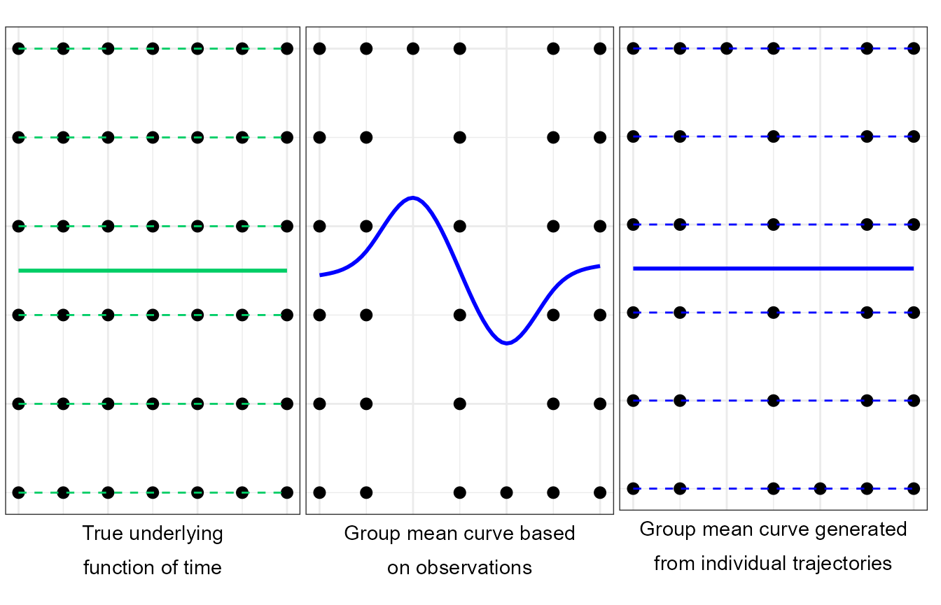

Multiple group mean curve fits (Center and Right) based on measurements generated from a true smooth underlying function of time (Left) with added inter-individual variability and missing observations. Multiple individual trajectories (Left, dashed green lines) are generated from a true underlying function of time (Left, continuous green line). Discrete measurements are generated (dots). Group mean curves are computed on a subset of these measurements (Center and Right, continuous blue line, 5 effective degrees of freedom). When the group mean curve is generated solely based on measurements (Center), the true underlying function of time is not satisfactorily approximated (fundamental unit of information is the observation). When the group mean curve (Right, continuous blue line) is generated from each individual curves (Right, dashed blue lines) a satisfactory approximation of the true underlying function of time can be obtained (fundamental unit of information is the functional representation of each individual).

Intra-class variability (confidence bands on the group mean curves)

Confidence bands are employed to represent the uncertainty in an function’s estimate based on limited or noisy data. Pointwise confidence bands on the group mean curve can therefore provide a visualisation of the variance of the overall mean function through time. The confidence bands indicate for each possible time, values of the mean curve which could have been produced by the provided individual trajectories, with at least a given probability.

As the underlying distribution of \(F(t)\) is unknown and inaccessible, confidence on \(g(t)\) must be estimated by sampling the approximate distribution available (i.e. the measurements), achieved by bootstrapping the observations¹³ ¹⁴ ¹⁵. Bootstrap assumes that sampling the distribution under a good estimate of the truth (the measurements) should be close to sampling the distribution under the true process. Once a bootstrapped distribution of mean curve is estimated, using the percentile method a pointwise confidence interval on \(g(t)\) can be calculated¹⁶ ¹⁷ ¹⁸ by taking the \(\alpha/2\) and \(1-\alpha/2\) quantiles at each time-point of interest (where \(\alpha\) is the error quantile in percent).

As limited assumptions on the fitted model can be established, empirical confidence bands on the group mean curve are calculated based on a non-parametric bootstrapped distribution. Individual curves are sampled with replacement and group mean curves calculated. The distribution of group mean curve is then employed to estimate the pointwise confidence bands.

Detection of significantly altered time-trajectories

With a continuous time representation of a metabolite’s concentration accessible (i.e. the group mean curve), a metric quantifying a global difference between such curves can be devised. This measure of difference, independent of the original sampling of the data (e.g. asynchronous and missing measurements), can then be employed to determine whether the group mean curves are identical across the two groups and calculate the significance of the result.

In order to identify time-trajectories that are significantly altered between two experimental groups \(G_1\) and \(G_2\), this global measure must be established. The measure must be able to detect baseline difference when both curves present the same shape, but also shape differences when the mean values across time are identical for both groups. We postulate that the area between two group mean curves fitted independently \(g_1(t)\) and \(g_2(t)\) (Eq. 3) is a good measure of the degree to which the two group time-trajectories differ. This global distance measure is calculated as:

\[dist(g_1,g_2) = \int_{t_{min}}^{t_{max}} |g_1(t)-g_2(t)| ~dt\] (Eq. 4)

Where:

\(t_{min}\) and \(t_{max}\) are the lower and upper bound of the time course.

The global distance measure is a quantification of evidence for differential time evolution, and the larger the value, the more the trajectories differ.

Given the groups \(G_1\), \(G_2\), their respective group mean curves \(g_1(t)\), \(g_2(t)\) and the observed global distance measure \(dist(g_1,g_2)\), the question of the significance of the difference between the two time trajectories is formulated as the following hypothesis-testing problem:

\(H_0\): \(g_1(t)\) and \(g_2(t)\) are identical.
\(H_1\): The two curves are not the same.

Under the null hypothesis \(H_0\), the global distance between \(g_1(t)\) and \(g_2(t)\) can be generated by a randomly permuting the individuals between two groups. Under the alternate hypothesis \(H_1\), the two curves are different, and very few random assignment of individuals to groups will generate group mean curves that differ more than the observed ones (i.e. a larger global distance).

In order to test the null hypothesis, the observed global distance must be compared to the expected global distance under the null hypothesis. The null distribution of the global distance measure is inferred by repeated permutations of the individual class labels¹⁹. Individual trajectories are fit using the chosen df and randomly assigned in one of two groups of size \(s_1\) and \(s_2\) (identical to the size of \(G_1\) and \(G_2\) respectively). The corresponding group mean curves \(g'_1(t)\) and \(g'_2(t)\) computed, and a global distance \(dist(g'_1,g'_2)\) calculated. This is repeated many times to form the null distribution of the global distance. From this distribution a \(p\)-value can be computed as the proportion of global distance as extreme or more extreme than the observed global distance (\(dist(g_1,g_2)\)). The \(p\)-value indicates the probability (if the null hypothesis was true) of a global difference as, or more, extreme than the observed one. If the \(p\)-value is inferior to an agreed significance level, the null hypothesis is rejected.

Due to the stochastic nature of the permutations, the null distribution sampled depends on the random draw, resulting in possible variation of the \(p\)-value. Variation on the permuted \(p\)-value can be described by confidence intervals. The \(p\)-value is considered as the success probability parameter \(p\) in \(n\) independent Bernoulli trials, where \(n=B\) the total number of permutation rounds²⁰. Confidence intervals on this binomial distribution of parameter \(p\) and \(n\) can then be computed. As extreme \(p\)-values are possible (i.e close to 0) and the number of permutation rounds could be small, the Wilson score interval²¹ is employed to determine the confidence intervals (Eq. 5):

\[p_\pm = \frac{1}{1+\frac{1}{B}z^2}\left ( p + \frac{1}{2B}z^2 \pm z\sqrt{\frac{1}{B} p (1 - p) + \frac{1}{4B^2}z^2 } \right )\] (Eq. 5)

Where:

\(p_\pm\) is the upper or lower confidence interval.
\(p\) is the calculated \(p\)-value.
\(B\) the total number of permutation rounds.
\(z\) is the \(1-1/2\alpha\) quantile of the standard normal distribution, with \(\alpha\) the error quantile.

Lastly, if a large number of variables are investigated for significantly altered trajectories, significance results must be corrected for multiple hypothesis testing. Here we employ the well-known Benjamini & Hochberg false discovery rate approach²² as default, with other methods available as an option.

Arnaud Wolfer

2019-10-03